Introduction

The Finite Element Method (FEM) is a technique to solve boundary value problems of partial differential equations numerically. These investigations shall provide a brief overview on aspects of a Quantum Finite Element Method (QFEM) already disputed and essentially focus on a very simple example of a boundary value problem to be solved via FEM and a quantum based linear solver. Similar to a broad range of algorithms in Machine Learning, the key step in the FEM consists in solving (large) systems of linear equations. In this connection, the application of quantum algorithms to solve the linear system instead of using classical numerical methods offers a potentially remarkable speedup.

The quantum way to solve linear systems

A so-called Quantum Linear System Algorithm (QLSA) is a method to solve a system of linear equations  in quantum sense whereat the input load vector  is prepared as a quantum state  and the solution is also delivered in form of a quantum state  corresponding to the solution of the classical linear system. The HHL algorithm is the most famous algorithm to solve a quantum linear system [1]. For the HHL algorithm the system matrix  has to be a quadratic hermitian matrix. We design our specific application scenario to cope with this condition. In general, it is also possible to reformulate the linear system to match these conditions. The basic idea of HHL is to solve the equation system via matrix inversion, which requires in quantum computing a feasible effort unlike in the classical sense. Therefore, the system matrix  is decomposed into a unitary matrix and a diagonal matrix, which contains the eigenvalues of  and is easy to invert. Figure 1 shows the three steps of the HHL algorithm: At first, the eigenvalues are determined using the Quantum Phase Estimation (QPE) [2] with the unitary  and a specific parameter . The second step applies a controlled rotation on an ancillary qubit. After reversing the QPE, the solution  is obtained if the ancillary qubit is measured as .

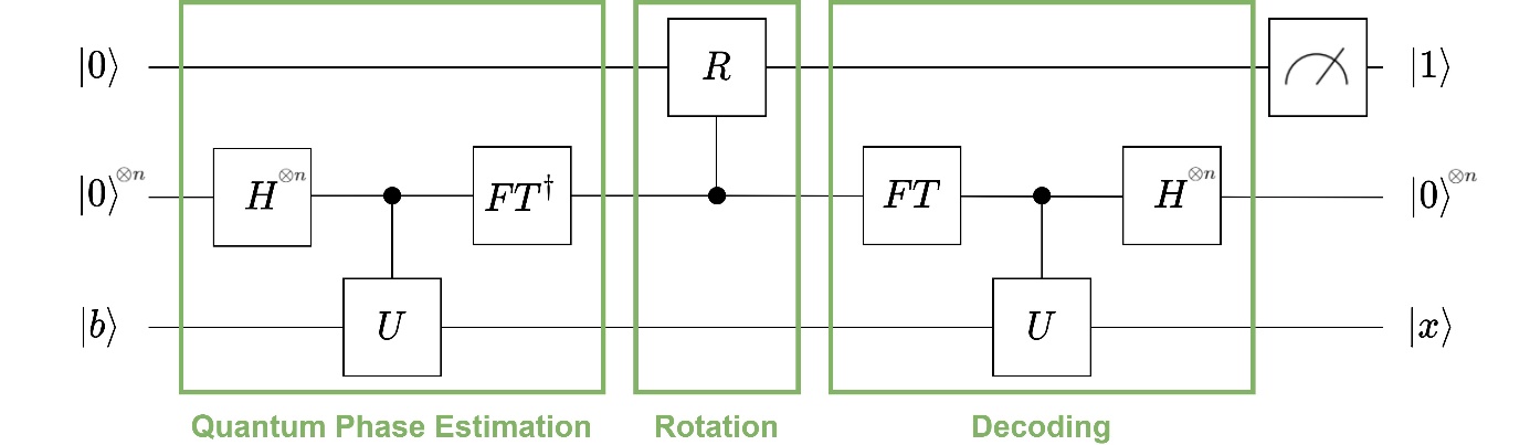
Figure 1: Steps of the HHL algorithm

There are several reasons why the FEM is a promising field of application for QLSA. On the one hand the large systems turning up in the FEM are generated algorithmically instead of directly being the input which avoids a need to access the data via quantum RAM [3]. On the other hand, the system assembling leads to sparse system matrices that are an important requirement when it comes to quantum speedup using a QLSA. Dependent on the specific application task, implementing a QLSA as part of the FEM routine allows potential polynomial speedups [4]. In the following, we refer to a simple 1D-setup as we consider a thin, cylindrical rod of length  and radius  (to allow 1D FEM). Furthermore we assume the rod to be connected with surrounding material holding a constant temperature . The rod is influenced by an external heat source, which temperature is described by a function  in space and time. The corresponding heat equation reads

whereat  is the rod’s temperature at position  and time  and  is the diffusivity constant depicting the thermal conductivity of the material the rod is made of. In analytical studies, this constant is often neglected because the constant can be simply added to our considerations afterwards. Hence, we set  for simplification but highlight that the specific value of this constant is very important in engineering aspects. We consider the steady-state solution of (1), which transfers the heat equation in a Poisson’s equation. Due to the described surrounding material, we add Dirichlet boundary conditions, which give us the boundary value problem

where we can neglect the temporal parameter. Figure 2 shows this stationary solution for a specific example of the problem (2) – (3).

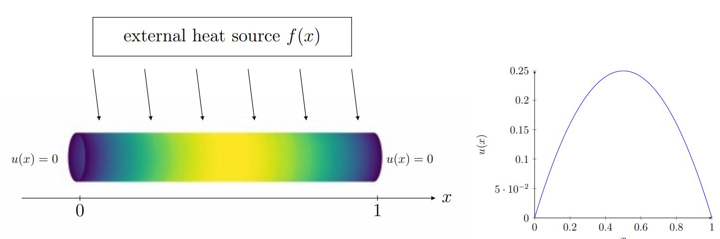
Figure 2: Analytic solution of the stationary Poisson’s equation with homogeneous Dirichlet boundary conditions with source term f(x)=2

Experiments on IBM quantum computers

For the calculations, we use various simulators as well as real quantum hardware (the IBM Q Melbourne) offering 15 qubits and a quantum volume of 8. We aim to test the very applicability of the HHL method as a quantum algorithm to solve the boundary value problem (2) – (3). We deploy solution plots for system sizes of ,  and , compare the approximation quality of the quantum algorithm dependent on system size and number of allocated qubits and determine the depth and width of the quantum circuits, which indicate the complexity of the quantum method. To evaluate the approximation quality we use a fidelity term, which describes the proximity of two quantum states and indicates the probability of identifying one of both status as the other one. Besides, we use the -distance between the classical solution and the solution given by the quantum procedure.

We identified a conflict between the amount of qubits provided for the quantum circuits, which naturally leads to an increased approximation quality of the quantum solution to the real solution (since the QPE-steps are proceeded with higher accuracy, see Figure 3), and the consequential complexity of the quantum circuit, depicted in Figure 4. Due to the limited number and quality of qubits in current real quantum hardware, a higher complexity causes errors in executing the circuit’s gates, which downgrade the quality of the quantum solution.

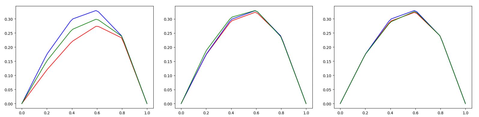
Figure 3: Increasing approximation quality of the quantum solution when providing more qubits for the HHL-circuit (Quantum Simulators and the expected curve (green) visualised)

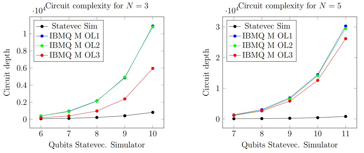
Figure 4: Deployment of the quantum circuit complexity at an increasing number of used qubits using different optimization levels for transpiling

In consequence, these opposing effects on the quality of the quantum solution result in an initial increase of the accuracy followed by a degradation due to the high circuit complexity when exceeding a certain amount of provided qubits.

Literature

[1] Harrow, A.W., Hassidim, A., and Lloyd, S., 2009. Quantum algorithm for solving linear systems of equations, Physical Review Letters 103(15).

[2] Nielsen, M.A., Chuang, I.L., 2011. Quantum computation and quantum information 10th anniversary edition (10th ed.), Cambridge University Press, NewYork, NY, USA.

[3] Aaronson, S., 2015. Quantum machine learning algorithms: Read the fine print, Nature Physics 11:291–293.

[4] Montanaro, A., and Pallister, S., 2015. Quantum algorithms and the finite element method, Physical Review A 93.

Introduction

Pattern recognition as one of the most common applications of machine learning is about the automatic discovery of regularities in data by a machine that uses computer algorithms for classification based on statistical information, historical data and memory. Commonly, machine learning methods for classification rely on neural networks, which contain a set of neurons that are ordered in several succeeding layers. Each of these neurons receives the results from the preceding layer as input arguments and provides an output defined by a certain activation function for the following layer. The inputs of a neuron are equipped with weights whose values are adapted by an optimization scheme during the training process, which consists in traversing training data with pre-labelled outcomes.

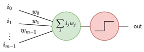
Figure 1: A neuron taking m input arguments and delivering output based on a threshold activation

A simple recognition problem

For a realisation of an artificial feed forward neural network on a quantum computer, we consider a simple recognition problem based on small “binary pictures”. The goal is to identify each picture with a pattern of two black pixels arranged one upon the other or side by side as illustrated by Figure 1. The considerations are based on the studies [1,2].

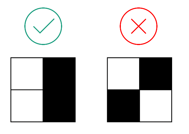
Figure 2: Visualisation of two binary images, whereof the left one represents the searched pattern

For this task we use a network, which consists of quantum artificial neurons – implementable on the IBM superconducting quantum processors. Each of the quantum neurons provide a potential advantage in storage capacity and is able to proceed classification tasks that are impossible to do via single classical nodes only. For classification problems, quantum computing provides a potential exponential speed-up.

Quantum neural network setup

The quantum neural network is embedded into a hybrid approach using quantum nodes, which take classical information as input and deliver a classical output. The quantum circuit for a single neuron is composed out of two encoding steps and the activation function as depicted by Figure 3.

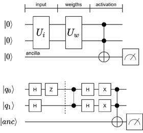
Figure 3: The circuit for a single quantum neuron with an exemplary realisation for a combination of image and weights
 

Since we focus on input images with four pixels, we need two qubits for the processing. An additional ancilla qubit receives and delivers the neuron’s output. Two unitary operations serve to encode the input arguments and the weights. The activation is proceeded via a multi-CNOT gate. The result can either be measured (as done in Figure 3) or passed through to further quantum neurons.

Finally, the target patterns distinguished from the other ones by delivering a probability amplitude of the state  greater that , which serves as the recognition threshold.

Literature

[1] Tacchino, F., Macchiavello, C., Gerace, D., and Bajoni, D., 2019. An artificial neuron implemented on an actual quantum processor, npj Quantum Information 5, 26.

[2] Tacchino, F., Barkoutsos, P., Macchiavello C., Tavernelli, I., Gerace D., and Bajoni D., 2020. Quantum implementation of an artificial feed-forward neural network, Quantum Science and Technology 5, 044010.

Introduction

Scheduling problems are a branch of combinatorial optimization problems. Thus, the objective is to optimize a schedule in terms of a target value. These schedules could be anything from landing sequences of aircrafts (a.k.a. aircraft landing problem) or sequences of work packages (a.k.a. job shop scheduling problem) to sequences of cars in a paint shop (e.g. binary paint shop problem). The target value would be in these cases e.g. landing the planes within their arrival time window, while maintaining safety distances, reducing the resources, or reducing the number of color swaps for a paint shop. While these problems are already formulated as mathematical models, in general this is not the case. Thus, the first step is to mathematically model the real-world problem. Once such a model is formulated it could be translated into different models. A model, which is suited for combinatorial optimization problems on universal gate-model quantum computers is the Ising-Hamiltonian and can be solved with the Quantum Approximate Optimization Algorithm (QAOA).

Quantum Approximate Optimization Algorithm

QAOA (“Quantum Approximate Optimization Algorithm” or “Quantum Alternating Operator Ansatz”) is a modern hybrid algorithm for the universal gate-model quantum computer. Its circuits are sparse and relatively shallow, which are both requirements for the execution on so-called NISQ-Devices (noisy intermediate-scale quantum computers) [1]. The term ‘hybrid’ refers here to the fact, that part of the algorithm is executed on a quantum computer and another part is executed on a classical computer. In fact, the circuits are parameterized and executed on the quantum computer. The classical computer is utilized to optimize the parameters using an optimization algorithm, which is either simplex or gradient based. Both parts are executed alternating until either optimal parameters are found, or other termination criteria are met. 

Figure 1: Quantum circuit diagram with QAOA Hamiltonians for p layers.

The binary paint shop problem

The binary paint shop problem is a simplification of real-world paint shops in the automotive industry, which Volkswagen has recently shown, that it is solvable with QAOA on a quantum computer [2]. The problem itself assumes, that there is a queue of car configurations which should be painted in one of two colors. Each car configuration exists twice in the queue and both configurations should be painted in opposite colors. The sequence of the cars can’t be changed. However, the algorithm can decide, if the first occurrence of a configuration should be colored with color one or color two. The second occurrence of the configuration is then, obviously, colored in the other color. It can be shown that already this simplification of the problem is not only NP-hard, but also APX-hard (there is no efficient algorithm, which can approximate the optimal solution).

Solving the binary paint shop problem with QAOA

To solve the binary paint shop problem with QAOA we have to convert the problem into a Hamiltonian. Here we will use the spin glass Hamiltonian, which is of the following form:

Each car configuration is only one qubit and  and  go over consecutive cars. If these cars are both either seen for the first time or seen for the second time  becomes  and otherwise . The mixing Hamiltonian is, as usual, of the following form:

The solution shows us then the color for the first occurrence of each car configuration.

Outlook

Volkswagen has shown, that a slight modification of the binary paint shop problem could be used to optimize the application of the primer in one of its car facilities [3]. However, this algorithm was executed on a quantum annealer.

Literature

[1] L. Zhou, S.-T. Wang, S. Choi, H. Pichler, und M. D. Lukin, „Quantum Approximate Optimization Algorithm: Performance, Mechanism, and Implementation on Near-Term Devices“, Phys. Rev. X, Bd. 10, Nr. 2, S. 021067, 2020, doi: 10.1103/PhysRevX.10.021067.

[2] M. Streif, S. Yarkoni, A. Skolik, F. Neukart, und M. Leib, „Beating classical heuristics for the binary paint shop problem with the quantum approximate optimization algorithm“, Nov. 2020, [Online]. Verfügbar unter: https://arxiv.org/pdf/2011.03403

[3] D-Wave Systems, Volkswagen: Paint Shop Optimization with Quantum Annealing, (Nov. 13, 2020). Zugegriffen: Apr. 15, 2021. [Online Video]. Verfügbar unter: https://www.youtube.com/embed/Uenk1SF8NsI

Introduction

Grover Adaptive Search (GAS) is an extension of the Grover Search (GS) algorithm. Instead of searching for a specific value, GAS can find the lowest (or highest) value without knowing the exact number before. Further, using a special initial state, namely the Quantum Dictionary, this allows us to find the optimal solution of combinatorial optimization problems using its QUBO representation. In this case study we want to examine Grover Adaptive Search on a specific combinatorial optimization problem, namely the problem of Portfolio Optimization.

Grover Search

Grover Search is an already older algorithm developed by Lov Grover in 1996 [1]. It utilizes Amplitude Amplification to find one or more entries in an unsorted set. The entry is a binary number and represented by the qubits. Thus, requiring one qubit per bit.

In general, the algorithm consists of multiple iterations, where one iteration consists of an oracle and a diffusion operator. Starting in an equal superposition over all entries, the oracle flags the entries of interest by inverting their amplitudes. The diffusion operator reflects then all amplitudes at the mean value of all amplitudes. This results in an overall higher amplitude of the entries of interest and a lower one of the others as shown in Figure 1. Applying the iterations, the amplitudes of the entries of interest are first rising, however there is a turning point, where it flips over resulting in lower amplitudes for the entries of interest. When we are looking only for one entry, we have to apply the  iterations, where  is the number of entries. Compared to the best-known classical algorithm we only need  instead of  runs.

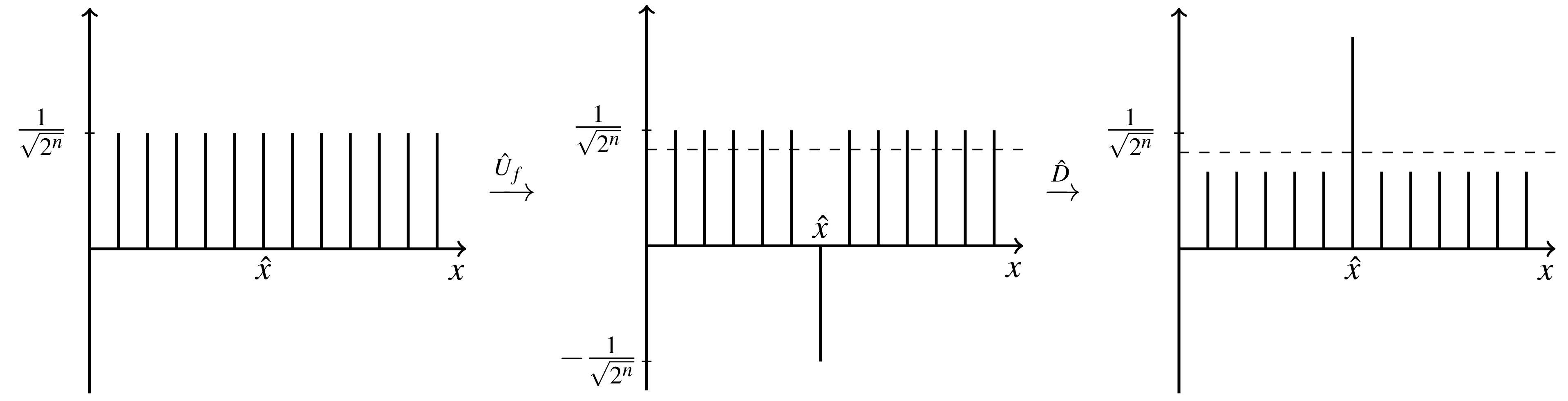
Figure 1: Demonstration of the effect of first applying the oracle and afterwards applying the diffusion operator.

On first sight this algorithm isn’t very useful, since we need to know the entries of interest in order to construct the oracle. However, using a Quantum Dictionary [2] we can extend Grover’s Algorithm to find a specific solution to a combinatorial optimization problem using QUBOs.

Quantum Dictionaries are maps of keys and values. They use a key and a value qubit register and store all entries in an equal superposition. Most importantly we don’t have to enter the value explicitly, but can use a function (e.g., a QUBO), that takes the key and calculates the value. Using Grover Search on the value register, we can now find a key (a combination of a combinatorial problem) for a specific value (a goal function value; the goal function is what we usually want to minimize or maximize). However, this leads us to a new problem since we usually don’t know the optimal goal function value in beforehand.

Grover Adaptive Search

Grover Adaptive Search solves the problem of finding a minimal or maximal value in a Quantum Dictionary using Grover Search [3]. For a minimization problem it starts with searching for all values, which are smaller than the highest value which can be represented by the value register or an educated guess. If the Grover Search has found a better value, we use this as our new boundary value. If we can’t find a better value after a given number of tries, we assume, that we have found the optimal value and its solution.

Portfolio Optimization

Portfolio Optimization tries to find an optimal subset of an investment universe in terms of risk and expected returns under a given budget.

As input, we have an investment universe of  assets, their expected returns  (as a vector) and a covariance matrix . Both can be calculated from historic values of the stock market. With a given risk appetite  we can create our object function , where  denotes, if we choose an asset or not. Usually, we have also a budget , which limits our ability to buy stocks. The budget is added to our object function as a penalty.

A Simple Portfolio Optimization Example

As an example, we use the stocks: GOOG, AAPL, TSLA and JPM, with their historic values from September 2021. We have a risk appetite of  and want to buy one quantity of two different stocks. A first glance at the relative historic values of our investment universe (see Figure 2) shows us already the optimal solution 0011 (0 – GOOG, 0 – AAPL, 1 – TSLA, 1 - JPM).

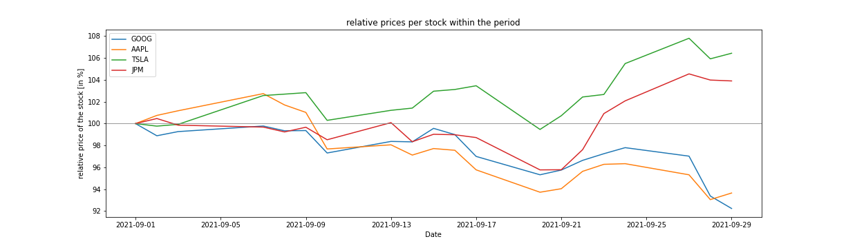
Figure 2: Comparison of the price trend in relative values for the  four stocks.

Without going too much into detail of the specific covariance matrix and the returns vector, we have to point out something important: Since we are using bit-values to represent the goal function value, we have to scale the matrix and the vector in such a way, that two goal function values are at least 1 apart from each other. However, this also effects the required number of qubits in the value register (the greater the number the more (qu)bits we need to represent them), thus we have to scale up very carefully.

We have executed 100 experiments for the given problem. Figure 3 shows, that we have a high probability to measure the correct result after executing Grover Adaptive Search. However, we have to admit, that we executed the experiments only on the state vector simulator and not on current hardware. This has two reasons: First, we already need for this small problem 12 fully connected qubits in a quantum computer and second, the current quantum computers are not able to execute quantum circuits with such a high depth (meaning the number of gates executed on one qubit).

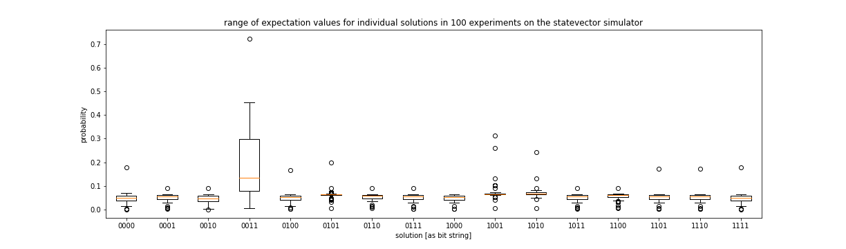
Figure 3: Results of 100 experiments Grover Adaptive Search on the Portfolio Optimization Problem (the optimal solution was 0011 and the budget was two).

Conclusion

In this case study we have shown how to solve the Portfolio Optimization Problem using Grover Adaptive Search. We have seen that Quantum Dictionaries and GAS are not viable on current Quantum Computers. However, we can use the same QUBO to solve the problem using QAOA or VQE. Further experiments have shown, that with a fault tolerant Quantum Computer with sufficient qubits GAS can outperform hybrid algorithms such as QAOA and VQE.

Literature

[1] L. K. Grover, “A fast quantum mechanical algorithm for database search,” ArXiv:quant-Ph9605043, Nov. 1996, Accessed: Oct. 11, 2021. [Online]. Available: http://arxiv.org/abs/quant-ph/9605043

[2] A. Gilliam et al., “Foundational Patterns for Efficient Quantum Computing,” ArXiv:190711513 Quant-Ph, Jan. 2021, Accessed: Apr. 15, 2021. [Online]. Available: http://arxiv.org/abs/1907.11513

[3] A. Gilliam, S. Woerner, and C. Gonciulea, “Grover Adaptive Search for Constrained Polynomial Binary Optimization,” ArXiv:191204088 Quant-Ph, Aug. 2020, Accessed: Mar. 01, 2021. [Online]. Available: http://arxiv.org/abs/1912.04088