Introduction

The Finite Element Method (FEM) is a technique to solve boundary value problems of partial differential equations numerically. These investigations shall provide a brief overview on aspects of a Quantum Finite Element Method (QFEM) already disputed and essentially focus on a very simple example of a boundary value problem to be solved via FEM and a quantum based linear solver. Similar to a broad range of algorithms in Machine Learning, the key step in the FEM consists in solving (large) systems of linear equations. In this connection, the application of quantum algorithms to solve the linear system instead of using classical numerical methods offers a potentially remarkable speedup.

The quantum way to solve linear systems

A so-called Quantum Linear System Algorithm (QLSA) is a method to solve a system of linear equations  in quantum sense whereat the input load vector  is prepared as a quantum state  and the solution is also delivered in form of a quantum state  corresponding to the solution of the classical linear system. The HHL algorithm is the most famous algorithm to solve a quantum linear system [1]. For the HHL algorithm the system matrix  has to be a quadratic hermitian matrix. We design our specific application scenario to cope with this condition. In general, it is also possible to reformulate the linear system to match these conditions. The basic idea of HHL is to solve the equation system via matrix inversion, which requires in quantum computing a feasible effort unlike in the classical sense. Therefore, the system matrix  is decomposed into a unitary matrix and a diagonal matrix, which contains the eigenvalues of  and is easy to invert. Figure 1 shows the three steps of the HHL algorithm: At first, the eigenvalues are determined using the Quantum Phase Estimation (QPE) [2] with the unitary  and a specific parameter . The second step applies a controlled rotation on an ancillary qubit. After reversing the QPE, the solution  is obtained if the ancillary qubit is measured as .

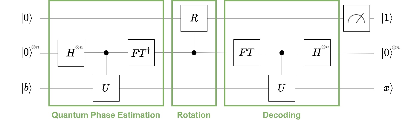
Figure 1: Steps of the HHL algorithm

There are several reasons why the FEM is a promising field of application for QLSA. On the one hand the large systems turning up in the FEM are generated algorithmically instead of directly being the input which avoids a need to access the data via quantum RAM [3]. On the other hand, the system assembling leads to sparse system matrices that are an important requirement when it comes to quantum speedup using a QLSA. Dependent on the specific application task, implementing a QLSA as part of the FEM routine allows potential polynomial speedups [4]. In the following, we refer to a simple 1D-setup as we consider a thin, cylindrical rod of length  and radius  (to allow 1D FEM). Furthermore we assume the rod to be connected with surrounding material holding a constant temperature . The rod is influenced by an external heat source, which temperature is described by a function  in space and time. The corresponding heat equation reads

whereat  is the rod’s temperature at position  and time  and  is the diffusivity constant depicting the thermal conductivity of the material the rod is made of. In analytical studies, this constant is often neglected because the constant can be simply added to our considerations afterwards. Hence, we set  for simplification but highlight that the specific value of this constant is very important in engineering aspects. We consider the steady-state solution of (1), which transfers the heat equation in a Poisson’s equation. Due to the described surrounding material, we add Dirichlet boundary conditions, which give us the boundary value problem

where we can neglect the temporal parameter. Figure 2 shows this stationary solution for a specific example of the problem (2) – (3).

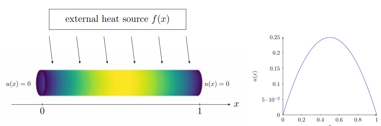
Figure 2: Analytic solution of the stationary Poisson’s equation with homogeneous Dirichlet boundary conditions with source term f(x)=2

Experiments on IBM quantum computers

For the calculations, we use various simulators as well as real quantum hardware (the IBM Q Melbourne) offering 15 qubits and a quantum volume of 8. We aim to test the very applicability of the HHL method as a quantum algorithm to solve the boundary value problem (2) – (3). We deploy solution plots for system sizes of ,  and , compare the approximation quality of the quantum algorithm dependent on system size and number of allocated qubits and determine the depth and width of the quantum circuits, which indicate the complexity of the quantum method. To evaluate the approximation quality we use a fidelity term, which describes the proximity of two quantum states and indicates the probability of identifying one of both status as the other one. Besides, we use the -distance between the classical solution and the solution given by the quantum procedure.

We identified a conflict between the amount of qubits provided for the quantum circuits, which naturally leads to an increased approximation quality of the quantum solution to the real solution (since the QPE-steps are proceeded with higher accuracy, see Figure 3), and the consequential complexity of the quantum circuit, depicted in Figure 4. Due to the limited number and quality of qubits in current real quantum hardware, a higher complexity causes errors in executing the circuit’s gates, which downgrade the quality of the quantum solution.

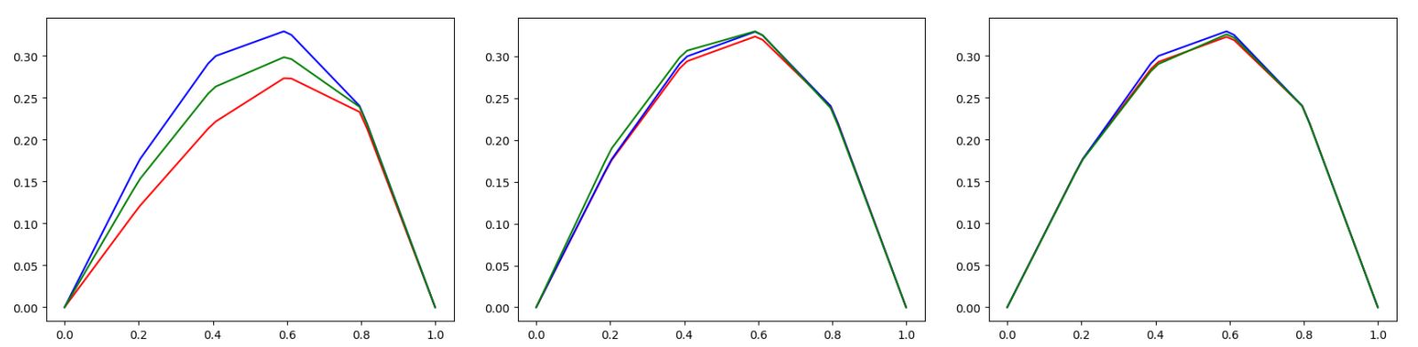
Figure 3: Increasing approximation quality of the quantum solution when providing more qubits for the HHL-circuit (Quantum Simulators and the expected curve (green) visualised)

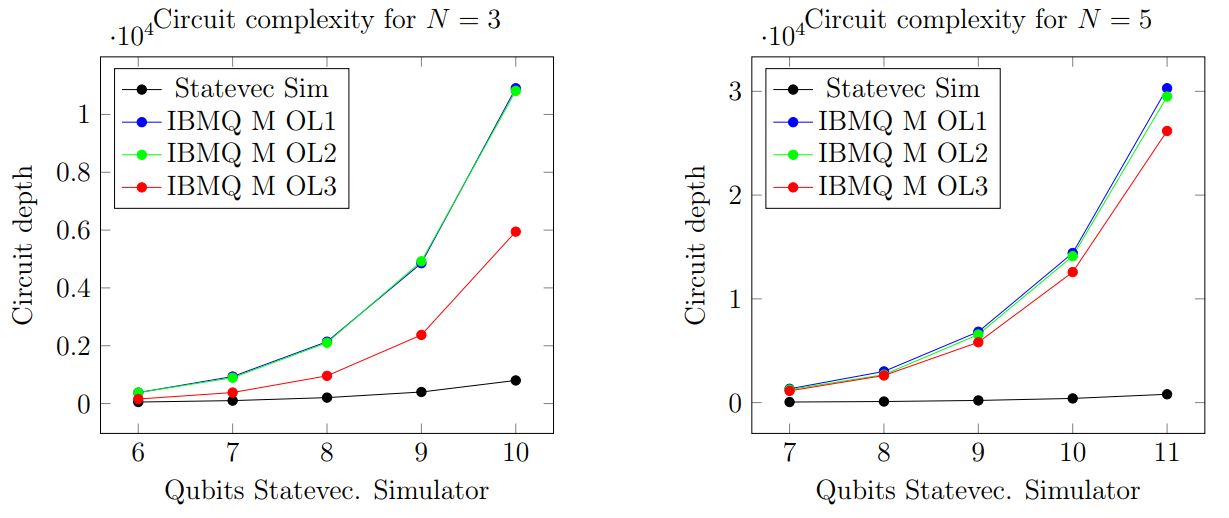
Figure 4: Deployment of the quantum circuit complexity at an increasing number of used qubits using different optimization levels for transpiling

In consequence, these opposing effects on the quality of the quantum solution result in an initial increase of the accuracy followed by a degradation due to the high circuit complexity when exceeding a certain amount of provided qubits.

Literature

[1] Harrow, A.W., Hassidim, A., and Lloyd, S., 2009. Quantum algorithm for solving linear systems of equations, Physical Review Letters 103(15).

[2] Nielsen, M.A., Chuang, I.L., 2011. Quantum computation and quantum information 10th anniversary edition (10th ed.), Cambridge University Press, NewYork, NY, USA.

[3] Aaronson, S., 2015. Quantum machine learning algorithms: Read the fine print, Nature Physics 11:291–293.

[4] Montanaro, A., and Pallister, S., 2015. Quantum algorithms and the finite element method, Physical Review A 93.